
RIVeR Tutorial
Introduction
RIVeR is a freeware that use displacement results from image velocimetry like PIV and PTV on oblique images in order to obtain superficial velocities. It can also be used to compute discharge of a river cross section; to obtain velocity components time-series or individual trajectories. The purpose of this tutorial is to show the complete process using the different software from a video to a discharge computation in a river cross section.
Setup
Since RIVeR is a compiled freeware made in the Matlab environment you should:
1) Download and install the Matlab Runtime version #R2015a (64-bit)
2) Download the last version of RIVeR
3)RIVeR uses results from image velocimetry software like PIVlab and PTVlab. They are both open-source software available on the Matworks file exchange platform. You must have a Matlab license in order to use them otherwise you can always contact me for a compiled version.
Case Study (discharge computation from a video with PIVlab and RIVeR)
Image Extraction
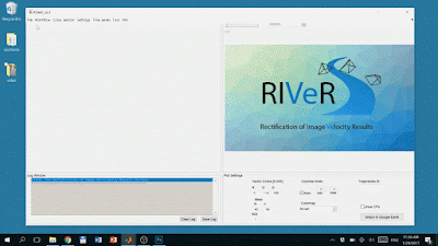
If you have recorded a video of a scene, you must extract the images of it in order to process them. Open RIVeR by double clicking on the RIVeR.exe inside its folder.
Go to File -> Extract Images from movie (Ctr-E). Select the video (the name of the file and its path should not include any space). Select the frame rate desired, the range that has to be processed (only a part of the recorded video might be interesting). Choose Grayscale in order to extract black and white images (increase the processing time). Images will be extracted in the same folder as the video.
Go to File -> Extract Images from movie (Ctr-E). Select the video (the name of the file and its path should not include any space). Select the frame rate desired, the range that has to be processed (only a part of the recorded video might be interesting). Choose Grayscale in order to extract black and white images (increase the processing time). Images will be extracted in the same folder as the video.

Image Processing (with PIVlab)
(text extracted from PIVlab - Tutorial)
You can now close RIVeR (we will get back to it after the image processing). Open PIVlab and Go to File -> New session. Click Load images in the panel that appears on the right side of the screen. Select the images you have extracted in the previous step. Set the sequencing style to 1-2, 2-3, 3-4, ... and click Add, then Import. The images are loaded in PIVlab. The image list on the panel on the right side displays the images that you selected. The letters 'A' & 'B' denote the first and the second image of one image pair (= one "frame"). In the lower right corner, you will find a slider to navigate through all frames, and a button (Toggle A/B) to toggle between the individual images within one frame.

Navigate to Analysis -> Analyze! and click Analyze all frames. You will see how the vector resolution increases with every pass.


You can now save the session. Select File -> Save -> PIVlab Session and close PIVlab. It is recomended to save the session in the same folder as the images. The resulting calculations consist of matrices or vectors of displacement for each pair of analyzed. images.
Load the results session in RIVeR
You can go back to RIVeR. To load the results session from the previus step, go to Workflow -> Load PIV /PTV analysis -> Load PIVlab / PTVlab session. Select the session file.

Load a background image
RIVeR doesn't rectifies the original images. It rectifies the results processed with PIVlab/PTVlab on the original images. However, in order to display the rectified results, a single image will be used as background. You can either pick one or make one automatically. Click on Workflow -> Load Background Image, choose Automatic.

Load a Control Points image
In order to rectify the results points with known coordinates in the real world need to be visible on the image. Those points are called Control Points (CPs), also known as Ground Reference Points. Thus, in order to rectify the results from the image processing, (at least) 4 four known CPs must be defined at the water surface plane. It should be noted that the CPs must not be co-aligned. In this example we will see how to use only 4 CPs that are in the same plane for results rectification. Click on Workflow -> Load CPs Image and select an image where all the CPs are visible (it might be the same as the Background Image).

Define CPs
In this step, we will define the CPs on the image and their position in the real world. Click on Workflow -> Define CPs -> Define in a 2D plane. You get to pick four (4) CPs on the image. It is preferred to select them counterclockwise and beginning by the CP on the left bank, upstream (in case of a river section). CPs are selected with the right click and zoom with left click.

Then, you are asked to define the real lengths between each CP. It is possible to import the lengths form a excel file or fill them manually in the following window. Select "Ok" when all the lenghts are filled.


The time between each image is defined by the frame rate (fps) used during the Image Extraction. It must be in [ms] and can be calculated as t = 1000/fps. In this example images have been extracted at 15 fps so the time between each image is t = 1000/15 = 66 ms.

Everything is set to rectify the results. Navigate to Workflow -> Rectify Results. It will take few seconds until the background image is rectified. The results of the first image pair is plotted on the right side of the interface. Now it is possible to navigate through all the results with the slider available. The last results will be the averaged velocity field. If you computed it in the Image Processing section the results number will be highlighted in green.


Define Region Of Interest
It is necessary to select a Region Of Interest (ROI) on the image. It is not the same region defined in PIVlab. It doesn't have to be a rectangular shape and it is preferable to choose a slightly larger ROI than the one chosen in PIVlab in order to have some areas without motion as ground reference. Build a polygon around the region you want to rectify and double-click on it. The area outside the ROI will be shaded.
Define time step
The time between each image is defined by the frame rate (fps) used during the Image Extraction. It must be in [ms] and can be calculated as t = 1000/fps. In this example images have been extracted at 15 fps so the time between each image is t = 1000/15 = 66 ms.

Rectify the results
Everything is set to rectify the results. Navigate to Workflow -> Rectify Results. It will take few seconds until the background image is rectified. The results of the first image pair is plotted on the right side of the interface. Now it is possible to navigate through all the results with the slider available. The last results will be the averaged velocity field. If you computed it in the Image Processing section the results number will be highlighted in green.

Discharge computation in a cross section
Cross Section Selection
Now that the results are rectified, make sure that the mean results are selected (highlighted in green). Go to Cross Section -> Add New -> On original image (left). Note, that it is also possible to define it on the rectified image (right). First, click on the left bank. A straight line will appear. Click on the right bank in order to define the cross-section. Once the cross-section is defined, double click on it to validate it's position, name it and click "Ok". A new window will pop-up where the velocity profile of the the selected cross-section is plotted. Only the streamwise component (perpendicular to the section) is used for the discharge computation.


Bathymetry Definition (with Areacomp2)
Areacomp2 is embedded in RIVeR 2.2 to facilitate the bathymetry definition of the Cross Section. AreaComp is usually used to analyze ADCP data and compute a relationship between channel area and stage for an ADCP measurement. It offers the possibility to import data from different ADCPs but also comma-separated value (CSV) data files. In the new window click on the button "AreaComp2" and the third window will popup. In this example, the bathymetry from an ADCP will be imported.
The bathymetry needs to be completed so it matches our Cross Section. Once completed go back to RIVeR. Navigate to File -> Go Back to RIVeR. Areacomp will close and the bathymetry will be imported directly to RIVeR. The discharge is computed using the mean-section method that consists in dividing the cross-section in N adjacent verticals at an equal distance d. Additionally, a coeficient between the superficial velocity and the mean velocity in the water column can be used. By default this coefficient is α=1.

Save/Export the results
Finally, the table can be copied to the clipboard in File -> Copy to clipboard. Close the current window and save. Go to File -> Project -> Save Project.

